Multiple Sclerosis
This data set was generated by Falcão et al, 2018 containing 2,208 mouse cells probed by SMART-seq2 with half experimental autoimmune encephalomyelitis (EAE) cells (in mimicing multiple scleorsis) and half control cells.
Here, we will illustrate how BRIE2 can be used to effectively detect differential splicing events between EAE and control cells, and using splicing ratio to predict cell type and disease conditions.
We have pre-processed the data with these BRIE2 scripts with brie-count and brie-quant. You can download the pre-computed data, e.g., by using the following command line and unzip it into the ./data folder for running this notebook.
wget http://ufpr.dl.sourceforge.net/project/brie-rna/examples/msEAE/brie2_msEAE.zip
unzip -j brie2_msEAE.zip -d ./data
Load Packages
[1]:
import umap
[2]:
import os
import brie
import numpy as np
import pandas as pd
import scanpy as sc
import matplotlib.pyplot as plt

print(brie.__version__)
2021-09-23 21:29:03.815258: W tensorflow/stream_executor/platform/default/dso_loader.cc:64] Could not load dynamic library 'libcudart.so.11.0'; dlerror: libcudart.so.11.0: cannot open shared object file: No such file or directory
2021-09-23 21:29:03.815359: I tensorflow/stream_executor/cuda/cudart_stub.cc:29] Ignore above cudart dlerror if you do not have a GPU set up on your machine.
2.0.6
[3]:
# define the path you store the example data
# dat_dir = "./data"
dat_dir = "/storage/yhhuang/research/brie2/releaseDat/msEAE/"
BRIE2 option 1: differential splicing events
Detecting differential splicing event by regressing on the EAE state with considering the strain covariate.
The command line is available at run_brie2.sh. Here is an example of design matrix besides the intercept and isEAE as the only testing variable.
samID   isEAE   isCD1
SRR7102862      0       1
SRR7103631      1       0
SRR7104046      1       1
SRR7105069      0       0
Besides the big .h5ad file, you can use the detected splicing events directely from brie_quant_cell.brie_ident.tsv. However, if you want get the quantify Psi for downstream analysis, e.g., option2 below, you need load the adata.layers['Psi'], and adata.layers['Psi_95CI'].
[4]:
adata = sc.read_h5ad(dat_dir + "/brie_quant_cell.h5ad")
adata
[4]:
AnnData object with n_obs × n_vars = 2208 × 3780
    obs: 'samID', 'samCOUNT'
    var: 'GeneID', 'GeneName', 'TranLens', 'TranIDs', 'n_counts', 'n_counts_uniq', 'loss_gene'
    uns: 'Xc_ids', 'brie_losses', 'brie_param', 'brie_version'
    obsm: 'Xc'
    varm: 'ELBO_gain', 'cell_coeff', 'effLen', 'fdr', 'intercept', 'p_ambiguous', 'pval', 'sigma'
    layers: 'Psi', 'Psi_95CI', 'Z_std', 'ambiguous', 'isoform1', 'isoform2', 'poorQual'
[5]:
adata.uns['brie_param']
[5]:
{'LRT_index': array([0]),
 'base_mode': 'full',
 'intercept_mode': 'gene',
 'layer_keys': array(['isoform1', 'isoform2', 'ambiguous'], dtype=object),
 'pseudo_count': 0.01}
Change gene index from Ensemebl id to gene name
[6]:
adata.var['old_index'] = adata.var.index
new_index = [adata.var.GeneName[i] + adata.var.GeneID[i][18:] for i in range(adata.shape[1])]
adata.var.index = new_index
[7]:
# if the index is bytes, change it to str

adata.var.index = [x.decode('utf-8') if type(x) == bytes else x for x in adata.var.index]
adata.obs.index = [x.decode('utf-8') if type(x) == bytes else x for x in adata.obs.index]
Add the cell annotations from input covariates
[8]:
adata.obs['MS'] = ['EAE' if x else 'Ctrl' for x in adata.obsm['Xc'][:, 0]]
adata.obs['isCD1'] = ['CD1_%d' %x for x in adata.obsm['Xc'][:, 1]]
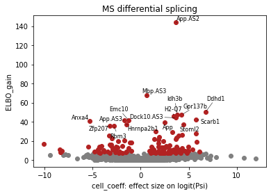
Volcano plot
Here, BRIE2 detects the differential splicing events between EAE and control. Cell_coeff means the effect size on logit(Psi). Positive value means higher Psi in isEAE.
[9]:
## volcano plot for differential splicing events
brie.pl.volcano(adata, y='ELBO_gain', log_y=False, n_anno=16, score_red=7, adjust=True)
plt.xlabel('cell_coeff: effect size on logit(Psi)')
plt.title("MS differential splicing")
[9]:
Text(0.5, 1.0, 'MS differential splicing')
[10]:
DSEs = adata.var.index[adata.varm['ELBO_gain'][:, 0] >= 7]
len(DSEs), len(np.unique([x.split('.')[0] for x in DSEs])), adata.shape
[10]:
(129, 123, (2208, 3780))
[11]:
adata.uns['Xc_ids']
[11]:
array(['isEAE', 'isCD1'], dtype=object)
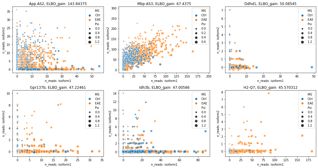
Visualize raw counts for DSEs
[12]:
rank_idx = np.argsort(adata.varm['ELBO_gain'][:, 0])[::-1]

fig = plt.figure(figsize=(15, 8))
brie.pl.counts(adata, genes=list(adata.var.index[rank_idx[:6]]),
               color='MS', add_val='ELBO_gain', ncol=3, alpha=0.7)
# fig.savefig(dat_dir + '../../figures/fig_s8_counts.png', dpi=300, bbox_inches='tight')
plt.show()
/home/yuanhua/MyGit/brie/brie/plot/base_plot.py:53: MatplotlibDeprecationWarning: Passing non-integers as three-element position specification is deprecated since 3.3 and will be removed two minor releases later.
  plt.subplot(nrow, ncol, i + 1)
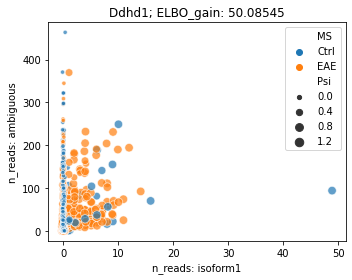
Changed ratio between ambiguous reads
Some differential splicing events having changed ratio on ambigous reads and isoform specific reads
[13]:
### Differential splicing shown by isoform1 and ambiguous reads

fig = plt.figure(figsize=(5, 4))
brie.pl.counts(adata, genes='Ddhd1',
               color='MS', add_val='ELBO_gain',
               layers=['isoform1', 'ambiguous'],
               nrow=1, alpha=0.7)
plt.show()
[ ]:
BRIE2 option 2: splicing quantification and usage
If you aim to use splicing isoform proportions as phenotypes for downstream analysis, e.g., to identify cell types, or study its disease contribution, we suggest not including the cell feature as covariate when quantifying Psi to avoid circular analysis.
Instead you could use gene level features, e.g., sequence features we introduced in BRIE1, or you can use an aggregated value from all cells as an informative prior. Similar as BRIE1, this prior is learned from the data and has a logit-normal distribution, so the information prior usually won’t be too strong.
In general, we recommend using the aggregation of cells as the prior thanks to its simplicity if it does not violate your biological hypothesis.
[14]:
adata_aggr = sc.read_h5ad(dat_dir + "/brie_quant_aggr.h5ad")

adata_aggr
[14]:
AnnData object with n_obs × n_vars = 2208 × 3780
    obs: 'samID', 'samCOUNT'
    var: 'GeneID', 'GeneName', 'TranLens', 'TranIDs', 'n_counts', 'n_counts_uniq'
    uns: 'brie_losses'
    obsm: 'Xc'
    varm: 'cell_coeff', 'effLen', 'intercept', 'p_ambiguous', 'sigma'
    layers: 'Psi', 'Psi_95CI', 'Z_std', 'ambiguous', 'isoform1', 'isoform2', 'poorQual'
[15]:
## change gene index
print(np.mean(adata.var['old_index'] == adata_aggr.var.index))

adata_aggr.var.index = adata.var.index
1.0
[16]:
# if the index is bytes, change it to str

adata_aggr.var.index = [x.decode('utf-8') if type(x) == bytes else x
                        for x in adata_aggr.var.index]
adata_aggr.obs.index = [x.decode('utf-8') if type(x) == bytes else x
                        for x in adata_aggr.obs.index]
Add meta data and gene-level annotation
Cell annotations and UMAP from gene-level expression. You can add any additional annotation.
[17]:
print(np.mean(adata.obs.index == adata_aggr.obs.index))
adata_aggr.obs['MS'] = adata.obs['MS'].copy()
adata_aggr.obs['isCD1'] = adata.obs['isCD1'].copy()
1.0
[18]:
dat_umap = np.genfromtxt(dat_dir + '/cell_X_umap.tsv', dtype='str', delimiter='\t')

mm = brie.match(adata_aggr.obs.index, dat_umap[:, 0])
idx = mm[mm != None].astype(int)

adata_aggr = adata_aggr[mm != None, :]
adata_aggr.obsm['X_GEX_UMAP'] = dat_umap[idx, 1:3].astype(float)
adata_aggr.obs['cluster'] = dat_umap[idx, 3]
adata_aggr.obs['combine'] = [adata_aggr.obs['cluster'][i] + '-' + adata_aggr.obs['MS'][i]
                            for i in range(adata_aggr.shape[0])]
[19]:
adata_aggr
[19]:
AnnData object with n_obs × n_vars = 1882 × 3780
    obs: 'samID', 'samCOUNT', 'MS', 'isCD1', 'cluster', 'combine'
    var: 'GeneID', 'GeneName', 'TranLens', 'TranIDs', 'n_counts', 'n_counts_uniq'
    uns: 'brie_losses'
    obsm: 'Xc', 'X_GEX_UMAP'
    varm: 'cell_coeff', 'effLen', 'intercept', 'p_ambiguous', 'sigma'
    layers: 'Psi', 'Psi_95CI', 'Z_std', 'ambiguous', 'isoform1', 'isoform2', 'poorQual'
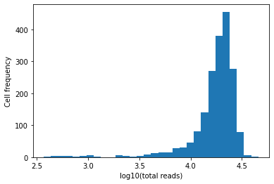
Cell filtering
[20]:
plt.hist(np.log10(adata_aggr.X.sum(1)[:, 0] + 1), bins=30)
plt.xlabel("log10(total reads)")
plt.ylabel("Cell frequency")
plt.show()
[21]:
# min_reads = 15000
min_reads = 3000

adata_aggr = adata_aggr[adata_aggr.X.sum(axis=1) > min_reads, :]
adata = adata[adata_aggr.obs.index, :]
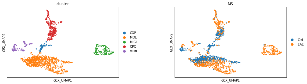
Visualizing splicing phenotypes in Gene expression UMAP
[22]:
sc.pl.scatter(adata_aggr, basis='GEX_UMAP', color=['cluster', 'MS'], size=30)
/home/yuanhua/.conda/envs/TFProb/lib/python3.7/site-packages/anndata/_core/anndata.py:1220: FutureWarning: The `inplace` parameter in pandas.Categorical.reorder_categories is deprecated and will be removed in a future version. Removing unused categories will always return a new Categorical object.
  c.reorder_categories(natsorted(c.categories), inplace=True)
/home/yuanhua/.conda/envs/TFProb/lib/python3.7/site-packages/anndata/_core/anndata.py:1229: ImplicitModificationWarning: Initializing view as actual.
  "Initializing view as actual.", ImplicitModificationWarning
Trying to set attribute `.obs` of view, copying.
... storing 'MS' as categorical
/home/yuanhua/.conda/envs/TFProb/lib/python3.7/site-packages/anndata/_core/anndata.py:1220: FutureWarning: The `inplace` parameter in pandas.Categorical.reorder_categories is deprecated and will be removed in a future version. Removing unused categories will always return a new Categorical object.
  c.reorder_categories(natsorted(c.categories), inplace=True)
Trying to set attribute `.obs` of view, copying.
... storing 'isCD1' as categorical
/home/yuanhua/.conda/envs/TFProb/lib/python3.7/site-packages/anndata/_core/anndata.py:1220: FutureWarning: The `inplace` parameter in pandas.Categorical.reorder_categories is deprecated and will be removed in a future version. Removing unused categories will always return a new Categorical object.
  c.reorder_categories(natsorted(c.categories), inplace=True)
Trying to set attribute `.obs` of view, copying.
... storing 'cluster' as categorical
/home/yuanhua/.conda/envs/TFProb/lib/python3.7/site-packages/anndata/_core/anndata.py:1220: FutureWarning: The `inplace` parameter in pandas.Categorical.reorder_categories is deprecated and will be removed in a future version. Removing unused categories will always return a new Categorical object.
  c.reorder_categories(natsorted(c.categories), inplace=True)
Trying to set attribute `.obs` of view, copying.
... storing 'combine' as categorical
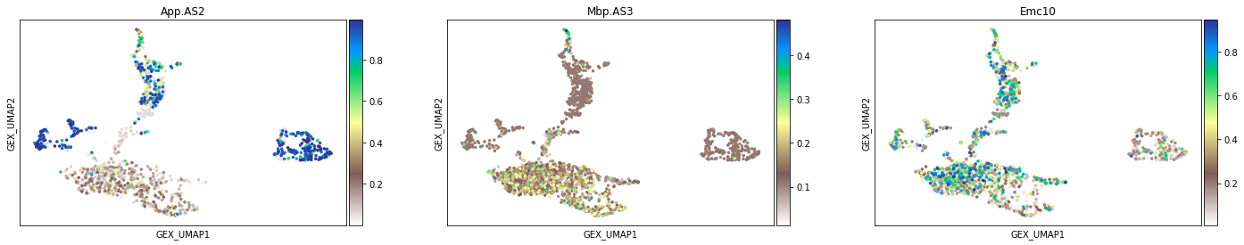
[23]:
sc.pl.scatter(adata_aggr, basis='GEX_UMAP', layers='Psi',
              color=['App.AS2', 'Mbp.AS3', 'Emc10'],
              size=50, color_map='terrain_r') #'terrain_r'
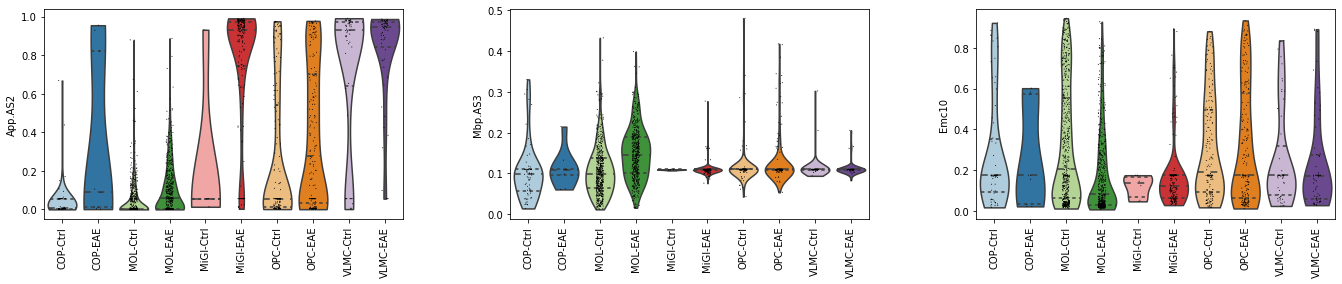
[24]:
import seaborn as sns

sc.pl.violin(adata_aggr, ['App.AS2', 'Mbp.AS3', 'Emc10'],
             layer='Psi', groupby='combine', rotation=90,
             inner='quartile', palette=sns.color_palette("Paired"))
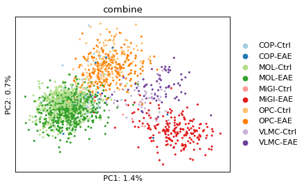
Dimension reduction on Psi
For downstream analysis, we only using splicing events that have been detected as differential splicing events. As mentioned earlier, the Psi is re-quantified by not using the cell-level information.
[25]:
# idx = list(adata.varm['fdr'][:, 0] < 0.05)
# adata_psi = adata_aggr[:, idx]

adata_psi = adata_aggr.copy()

adata_psi.layers['X'] = adata_psi.X.astype(np.float64)
adata_psi.X = adata_psi.layers['Psi']
adata_psi.shape
[25]:
(1845, 3780)
[26]:
sc.tl.pca(adata_psi, svd_solver='arpack')
[27]:
adata_psi.obs['Psi_PC1'] = adata_psi.obsm['X_pca'][:, 0]
adata_psi.obs['Psi_PC2'] = adata_psi.obsm['X_pca'][:, 1]
adata_psi.obs['Psi_PC3'] = adata_psi.obsm['X_pca'][:, 2]
[28]:
fig = plt.figure(figsize=(5, 3.7), dpi=80)
ax = plt.subplot(1, 1, 1)
sc.pl.pca(adata_psi, color='combine', size=30, show=False, ax=ax,
          palette=sns.color_palette("Paired"))
plt.xlabel("PC1: %.1f%%" %(adata_psi.uns['pca']['variance_ratio'][0] * 100))
plt.ylabel("PC2: %.1f%%" %(adata_psi.uns['pca']['variance_ratio'][1] * 100))
# plt.legend(loc=1)
plt.show()
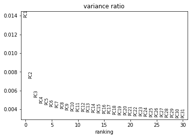
[29]:
sc.pl.pca_variance_ratio(adata_psi)
[30]:
sc.pp.neighbors(adata_psi, n_neighbors=10, n_pcs=20, method='umap')
sc.tl.umap(adata_psi)
/home/yuanhua/.conda/envs/TFProb/lib/python3.7/site-packages/numba/np/ufunc/parallel.py:363: NumbaWarning: The TBB threading layer requires TBB version 2019.5 or later i.e., TBB_INTERFACE_VERSION >= 11005. Found TBB_INTERFACE_VERSION = 6103. The TBB threading layer is disabled.
  warnings.warn(problem)
OMP: Info #271: omp_set_nested routine deprecated, please use omp_set_max_active_levels instead.
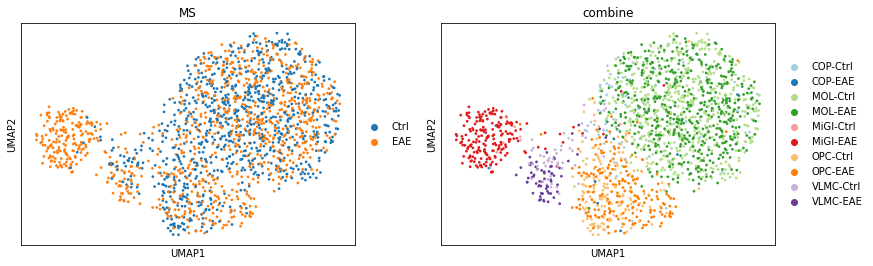
[31]:
sc.pl.umap(adata_psi, color=['MS', 'combine'], size=30)
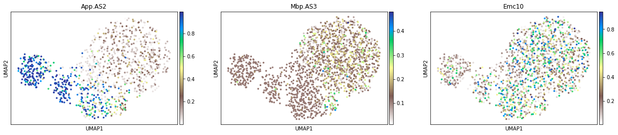
Visualise the Psi value on Psi-based UMAP
[32]:
sc.pl.umap(adata_psi, color=['App.AS2', 'Mbp.AS3', 'Emc10'], size=50, cmap='terrain_r')
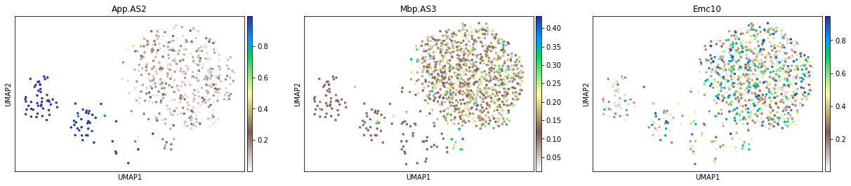
Only for the cells with confident Psi estimate
[33]:
adata_tmp = adata_psi[adata_psi[:, 'App.AS2'].layers['Psi_95CI'] < 0.3, :]
adata_tmp.X = adata_tmp.layers['Psi']
sc.pl.umap(adata_tmp, color=['App.AS2', 'Mbp.AS3', 'Emc10'], size=50, cmap='terrain_r')
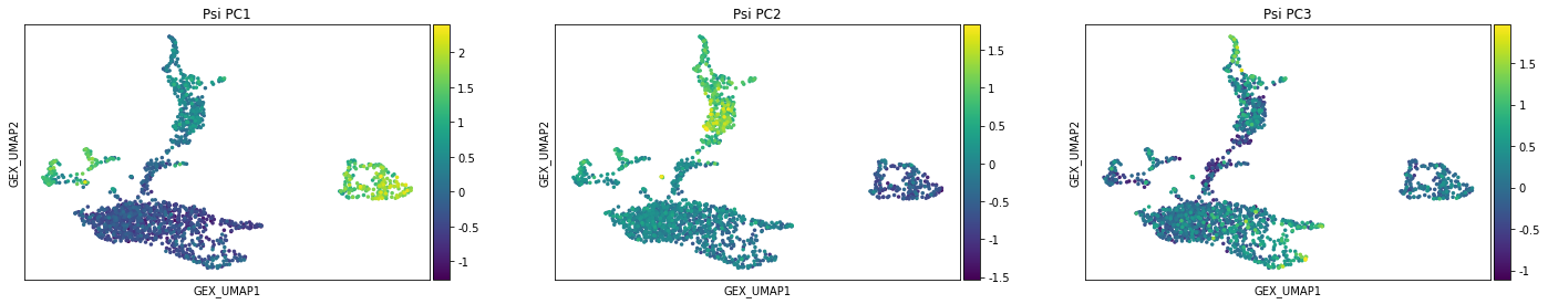
[34]:
sc.pl.scatter(adata_psi, basis='GEX_UMAP', color=['Psi_PC1', 'Psi_PC2', 'Psi_PC3'], size=50)
[ ]:
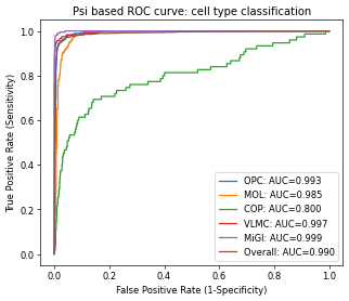
Prediction of cell type
One potential usage of the quantified Psi is to identify cell types. Instead of using them to cluster cells, here we show that by using the Psi (and their principle compoments), the annotated cell types from gene expression can be accurately predicted.
[35]:
np.random.seed = 1
[36]:
_val, _idx = np.unique(pd.factorize(adata_psi.obs['cluster'])[0], return_index=True)
print(_val, _idx)
print(adata_psi.obs['cluster'][_idx])
[0 1 2 3 4] [  0   8  54  92 890]
SRR7102862     OPC
SRR7102870     MOL
SRR7102925     COP
SRR7102967    VLMC
SRR7103970    MiGl
Name: cluster, dtype: category
Categories (5, object): ['COP', 'MOL', 'MiGl', 'OPC', 'VLMC']
[37]:
import scipy.stats as st
from sklearn import linear_model
from sklearn.ensemble import RandomForestClassifier
from hilearn import ROC_plot, CrossValidation

LogisticRegression = linear_model.LogisticRegression()
RF_class = RandomForestClassifier(n_estimators=100, n_jobs=-1)

X1 = adata_psi.obsm['X_pca'][:, :20]
Y1 = pd.factorize(adata_psi.obs['cluster'])[0]

CV = CrossValidation(X1, Y1)
# Y1_pre, Y1_score = CV.cv_classification(model=RF_class, folds=10)
Y2_pre, Y2_score = CV.cv_classification(model=LogisticRegression, folds=10)
[38]:
fig = plt.figure(figsize=(6, 5), dpi=60)
# ROC_plot(Y1, Y1_score[:,1], label="Random Forest", base_line=False)
# ROC_plot(Y1, Y2_score[:,1], label="Logistic Regress")

for i in range(5):
    ROC_plot(Y1 == i, Y2_score[:,i],
             legend_label=adata_psi.obs['cluster'][_idx[i]],
             base_line=False)
ROC_plot(np.concatenate([Y1 == i for i in range(5)]),
         Y2_score.T.reshape(-1), legend_label='Overall')

plt.title("Psi based ROC curve: cell type classification")

# fig.savefig(dat_dir + '../../figures/fig_s7_classification.pdf', dpi=300, bbox_inches='tight')
plt.show()
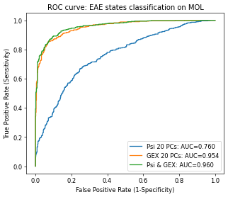
Prediction of MS state
Besides using Psi to predict the cell types, a more interesting task is to predict if a cell is in disease state (i.e., EAE state). Though by only using the Psi, it achieves moderate performance but clearly improves the prediction together with the gene expression.
[39]:
dat_GEX_pc = np.genfromtxt(dat_dir + 'top_20PC.tsv', dtype='str', delimiter='\t')
[40]:
idx = brie.match(adata_psi.obs.index, dat_GEX_pc[:, 0])
GEX_pc = dat_GEX_pc[idx, 1:].astype(float)
[41]:
adata_psi
[41]:
AnnData object with n_obs × n_vars = 1845 × 3780
    obs: 'samID', 'samCOUNT', 'MS', 'isCD1', 'cluster', 'combine', 'Psi_PC1', 'Psi_PC2', 'Psi_PC3'
    var: 'GeneID', 'GeneName', 'TranLens', 'TranIDs', 'n_counts', 'n_counts_uniq'
    uns: 'brie_losses', 'cluster_colors', 'MS_colors', 'pca', 'combine_colors', 'neighbors', 'umap'
    obsm: 'Xc', 'X_GEX_UMAP', 'X_pca', 'X_umap'
    varm: 'cell_coeff', 'effLen', 'intercept', 'p_ambiguous', 'sigma', 'PCs'
    layers: 'Psi', 'Psi_95CI', 'Z_std', 'ambiguous', 'isoform1', 'isoform2', 'poorQual', 'X'
    obsp: 'distances', 'connectivities'
[42]:
np.random.RandomState(0)
[42]:
RandomState(MT19937) at 0x7F09201C87C0
[43]:
import scipy.stats as st
from sklearn import linear_model
from hilearn import ROC_plot, CrossValidation

# np.random.seed(0)

X1 = adata_psi.obsm['X_pca'][:, :20]
X2 = GEX_pc
X3 = np.append(GEX_pc, adata_psi.obsm['X_pca'][:, :20], axis=1)
Y1 = pd.factorize(adata_psi.obs['MS'])[0]

X1 = X1[adata_psi.obs['cluster'] == 'MOL']
X2 = X2[adata_psi.obs['cluster'] == 'MOL']
X3 = X3[adata_psi.obs['cluster'] == 'MOL']
Y1 = Y1[adata_psi.obs['cluster'] == 'MOL']

LogisticRegression = linear_model.LogisticRegression(max_iter=5000)
CV = CrossValidation(X1, Y1)
Y1_pre, Y1_score = CV.cv_classification(model=LogisticRegression, folds=10)

LogisticRegression = linear_model.LogisticRegression(max_iter=5000)
CV = CrossValidation(X2, Y1)
Y2_pre, Y2_score = CV.cv_classification(model=LogisticRegression, folds=10)

LogisticRegression = linear_model.LogisticRegression(max_iter=5000)
CV = CrossValidation(X3, Y1)
Y3_pre, Y3_score = CV.cv_classification(model=LogisticRegression, folds=10)
[44]:
fig = plt.figure(figsize=(6, 5), dpi=60)
ROC_plot(Y1, Y1_score[:,1], label="Psi 20 PCs", base_line=False)
ROC_plot(Y1, Y2_score[:,1], label="GEX 20 PCs", base_line=False)
ROC_plot(Y1, Y3_score[:,1], label="Psi & GEX")

plt.title("ROC curve: EAE states classification on MOL")

# fig.savefig(dat_dir + '../../figures/fig_s9_EAE_predict.pdf', dpi=300, bbox_inches='tight')
plt.show()
Warning: label argument is replaced by legend_label and will be moved in future
Warning: label argument is replaced by legend_label and will be moved in future
Warning: label argument is replaced by legend_label and will be moved in future
[ ]:
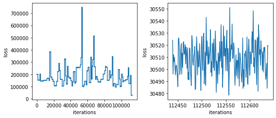
Techinical diagnosis
[45]:
## There are multiple batches in running jobs, so you will steps;
## the second part shows the last bit of the final batch

brie.pl.loss(adata.uns['brie_losses'])
[ ]: