scNT-seq
scNT-seq (Qiu, Hu, et al 2020) is a recently proposed technique to metabolically label newly synthesied RNAs in single cells. By using the labelling information, the inferred cellular transitions by Dynamo are hihgly consistent with the stimulation time (see our reproduced analysis with scripts from the authors).
This relative-longe-period transition is generally difficult to be obtained from RNA velocity by only using total RNAs. Here, we will illustrate that the differential momentum genes could help correct the projected trajectory, thanks to using the stimulation time as a testing (i.e., supervised) covariate.
As BRIE2 takes ~30 minutes with GPU to detect the DMGs, we provide the pre-computed data with these BRIE2 scripts. You can run this notebook by downloading the data, e.g., using the following command line and unzip it into the ./data folder:
wget http://ufpr.dl.sourceforge.net/project/brie-rna/examples/scNTseq/brie2_scNTseq.zip
unzip -j brie2_scNTseq.zip -d ./data
Load packages
[1]:
import brie
import numpy as np
import scanpy as sc
import scvelo as scv
import matplotlib.pyplot as plt
scv.logging.print_version()
Running scvelo 0.2.1 (python 3.7.6) on 2020-11-06 11:33.
WARNING: There is a newer scvelo version available on PyPI:
 Your version:           0.2.1
 Latest version:         modeling
[2]:
scv.settings.verbosity = 3  # show errors(0), warnings(1), info(2), hints(3)
scv.settings.presenter_view = True  # set max width size for presenter view
scv.set_figure_params('scvelo')  # for beautified visualization
[3]:
# define the path you store the example data
dat_dir = "./data"
# dat_dir = '/storage/yhhuang/research/brie2/releaseDat/scNTseq/'
scVelo dynamical model with total RNAs
This may take a few minutes to run, so we provide the pre-computed the data as in the above zip file for the setting with top 2,000 genes. The commented Python scripts are below. You can get the neuron_splicing_totalRNA.h5ad from here generated by the adapted script. If you want to change to more hihgly variable genes, you can change n_top_genes to other value, e.g., 8000.
adata = scv.read(dat_dir + "/neuron_splicing_totalRNA.h5ad")

scv.pp.filter_and_normalize(adata, min_shared_counts=30, n_top_genes=2000)
scv.pp.moments(adata, n_pcs=30, n_neighbors=30)

scv.tl.recover_dynamics(adata, var_names='all')
scv.tl.velocity(adata, mode='dynamical')
scv.tl.velocity_graph(adata)
scv.tl.latent_time(adata)
adata.write(dat_dir + "/scvelo_neuron_totalRNA_dynamical_2K.h5ad")
Cellular transitions on default selected velocity genes
[4]:
adata = scv.read(dat_dir + "/scvelo_neuron_totalRNA_dynamical_2K.h5ad")

print(adata.shape, np.sum(adata.var['velocity_genes']))
adata
(3066, 1999) 132
[4]:
AnnData object with n_obs × n_vars = 3066 × 1999
    obs: 'cellname', 'time', 'early', 'late', 'initial_size_spliced', 'initial_size_unspliced', 'initial_size', 'n_counts', 'velocity_self_transition', 'root_cells', 'end_points', 'velocity_pseudotime', 'latent_time'
    var: 'gene_short_name', 'gene_count_corr', 'means', 'dispersions', 'dispersions_norm', 'fit_alpha', 'fit_beta', 'fit_gamma', 'fit_t_', 'fit_scaling', 'fit_std_u', 'fit_std_s', 'fit_likelihood', 'fit_u0', 'fit_s0', 'fit_pval_steady', 'fit_steady_u', 'fit_steady_s', 'fit_variance', 'fit_alignment_scaling', 'fit_r2', 'velocity_genes'
    uns: 'neighbors', 'pca', 'recover_dynamics', 'velocity_graph', 'velocity_graph_neg', 'velocity_params'
    obsm: 'X_pca', 'X_umap'
    varm: 'PCs', 'loss'
    layers: 'Ms', 'Mu', 'fit_t', 'fit_tau', 'fit_tau_', 'spliced', 'unspliced', 'velocity', 'velocity_u'
    obsp: 'connectivities', 'distances'
[5]:
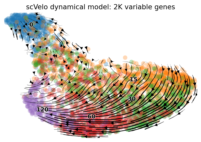
scv.pl.velocity_embedding_stream(adata, basis='umap', color=['time'],
                                 ax=None, show=True, legend_fontsize=10, dpi=80,
                                 title='scVelo dynamical model: 2K variable genes')
computing velocity embedding
    finished (0:00:00) --> added
    'velocity_umap', embedded velocity vectors (adata.obsm)
For 8K top variable genes
You can skip this sub section if not using the 8K top genes
adata2 = scv.read(dat_dir + "/scvelo_neuron_totalRNA_dynamical_8K.h5ad")
print(adata2.shape, np.sum(adata2.var['velocity_genes']))

scv.pl.velocity_embedding_stream(adata2, basis='umap', color=['time'],
                                 ax=None, show=True, legend_fontsize=10,
                                 title='scVelo dynamical model: 8K variable genes')
BRIE2 for differential momentum genes (DMGs)
Besides the large h5ad file, BRIE2 also saves the DMGs in a .tsv file brie_neuron_splicing_time.brie_ident.tsv for quick access.
[6]:
adata_brie = scv.read(dat_dir + "/brie_neuron_splicing_time.h5ad")

adata_brie
[6]:
AnnData object with n_obs × n_vars = 3066 × 7849
    obs: 'cellname', 'time', 'early', 'late'
    var: 'gene_short_name', 'n_counts', 'n_counts_uniq', 'loss_gene'
    uns: 'Xc_ids', 'brie_losses', 'brie_param', 'brie_version'
    obsm: 'X_umap', 'Xc'
    varm: 'ELBO_gain', 'cell_coeff', 'fdr', 'intercept', 'pval', 'sigma'
    layers: 'Psi', 'Psi_95CI', 'Z_std', 'spliced', 'unspliced'
[7]:
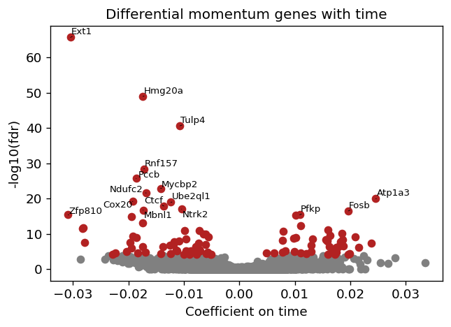
fig = plt.figure(figsize=(6, 4), dpi=60)
brie.pl.volcano(adata_brie, y='fdr', n_anno=16, adjust=True)
plt.title('Differential momentum genes with time')
plt.xlabel('Coefficient on time')
# plt.savefig(dat_dir + '../../figures/scNT_volcano.png', dpi=300)
plt.show()
RNA velocity on DMGs
[8]:
idx = (np.min(adata_brie.varm['fdr'], axis=1) < 0.01)
gene_use = adata_brie.var.index[idx]
print(sum(idx), sum(brie.match(gene_use, adata.var.index) != None))
n_genes = sum(brie.match(gene_use, adata.var.index) != None)
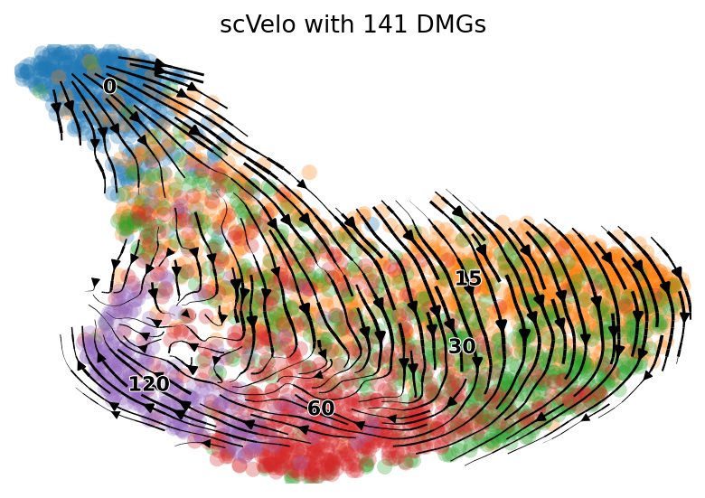
scv.tl.velocity_graph(adata, gene_subset=gene_use)
scv.pl.velocity_embedding_stream(adata, basis='umap', color=['time'],
legend_fontsize=10,
ax=None, show=True, dpi=80,
title='scVelo with %d DMGs' %(n_genes))
280 141
computing velocity graph
    finished (0:00:01) --> added
    'velocity_graph', sparse matrix with cosine correlations (adata.uns)
computing velocity embedding
    finished (0:00:00) --> added
    'velocity_umap', embedded velocity vectors (adata.obsm)
Change cutoffs
[9]:
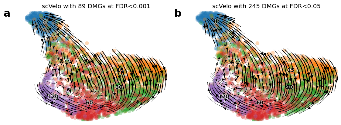
fig = plt.figure(figsize=(11, 4), dpi=60)
## cutoff 0.001
ax1 = plt.subplot(1, 2, 1)

idx1 = (np.min(adata_brie.varm['fdr'], axis=1) < 0.001)
gene_use1 = adata_brie.var.index[idx1]
n_gene1 = sum(brie.match(gene_use1, adata.var.index) != None)

print(sum(idx1), n_gene1)

scv.tl.velocity_graph(adata, gene_subset=gene_use1)
scv.pl.velocity_embedding_stream(adata, basis='umap', color=['time'],
                                 ax=ax1, show=False, legend_fontsize=10,
                                 title='scVelo with %d DMGs at FDR<0.001' %(n_gene1))
ax1.text(-0.15, 0.95, 'a', transform=ax1.transAxes, size=20, weight='bold')


## cutoff 0.05
ax2 = plt.subplot(1, 2, 2)
idx2 = (np.min(adata_brie.varm['fdr'], axis=1) < 0.05)
gene_use2 = adata_brie.var.index[idx2]
n_gene2 = sum(brie.match(gene_use2, adata.var.index) != None)

print(sum(idx2), n_gene2)

scv.tl.velocity_graph(adata, gene_subset=gene_use2)
scv.pl.velocity_embedding_stream(adata, basis='umap', color=['time'],
                                 ax=ax2, show=False, legend_fontsize=10,
                                 title='scVelo with %d DMGs at FDR<0.05' %(n_gene2))
ax2.text(-0.15, 0.95, 'b', transform=ax2.transAxes, size=20, weight='bold')

# plt.tight_layout()
# plt.savefig(dat_dir + '../../figures/scNT_scVelo_brie_FDR.png', dpi=300)
# plt.show()
165 89
computing velocity graph
    finished (0:00:01) --> added
    'velocity_graph', sparse matrix with cosine correlations (adata.uns)
computing velocity embedding
    finished (0:00:00) --> added
    'velocity_umap', embedded velocity vectors (adata.obsm)
516 245
computing velocity graph
    finished (0:00:02) --> added
    'velocity_graph', sparse matrix with cosine correlations (adata.uns)
computing velocity embedding
    finished (0:00:00) --> added
    'velocity_umap', embedded velocity vectors (adata.obsm)
[9]:
Text(-0.15, 0.95, 'b')
Visualize gene count
[10]:
idx = (np.min(adata_brie.varm['fdr'], axis=1) < 0.1)
gene_use = adata_brie.var.index[idx]

mm = brie.match(gene_use, adata.var.index) != None
gene_use[mm]
[10]:
Index(['Ncor1', 'App', 'Meis2', 'Tcf12', 'Elavl4', 'Cdk2ap1', 'Usp24', 'Ahi1',
       'Zfp608', 'Meaf6',
       ...
       'Zbtb11', 'Pdpk1', 'Pccb', 'Frem2', 'Sap18', 'Celf4', 'St6gal1',
       'Zfp704', 'Zkscan1', 'Mpp6'],
      dtype='object', length=319)
[11]:
## sorted by fdr
idx_sort = np.argsort(adata_brie[:, gene_use[mm]].varm['fdr'][:,0])
gene_use[mm][idx_sort]
[11]:
Index(['Ext1', 'Pccb', 'Ube2ql1', 'Ntrk2', 'Mbnl1', 'Fosb', 'Pfkp', 'Orc5',
       'Srd5a1', 'Chka',
       ...
       'Tjp1', 'Hivep3', 'Zkscan1', 'Mthfd1l', 'Prrc2c', 'Mllt3', 'Pdpk1',
       'St6gal1', 'Ktn1', 'Prkcb'],
      dtype='object', length=319)
[12]:
## Only negative coefficient
gene_sorted = gene_use[mm][idx_sort]
gene_sorted[adata_brie[:, gene_sorted].varm['cell_coeff'][:, 0] < 0]
[12]:
Index(['Ext1', 'Pccb', 'Ube2ql1', 'Ntrk2', 'Mbnl1', 'Orc5', 'Srd5a1', 'Akap9',
       'Ank2', 'Dlgap1',
       ...
       'Gmds', 'Satb2', 'Tjp1', 'Hivep3', 'Zkscan1', 'Mthfd1l', 'Prrc2c',
       'Mllt3', 'St6gal1', 'Ktn1'],
      dtype='object', length=212)
[13]:
## Only positive coefficient
gene_sorted = gene_use[mm][idx_sort]
gene_sorted[adata_brie[:, gene_sorted].varm['cell_coeff'][:, 0] > 0]
[13]:
Index(['Fosb', 'Pfkp', 'Chka', 'Homer1', 'Erf', 'Nup98', 'Ncapg2', 'Ifrd1',
       'Rasgef1b', 'Tiparp',
       ...
       '1810030O07Rik', 'Jmy', 'Slc3a2', 'Kcnq5', 'Stx5a', 'Clk4', 'Fbl',
       'Sap18', 'Pdpk1', 'Prkcb'],
      dtype='object', length=107)
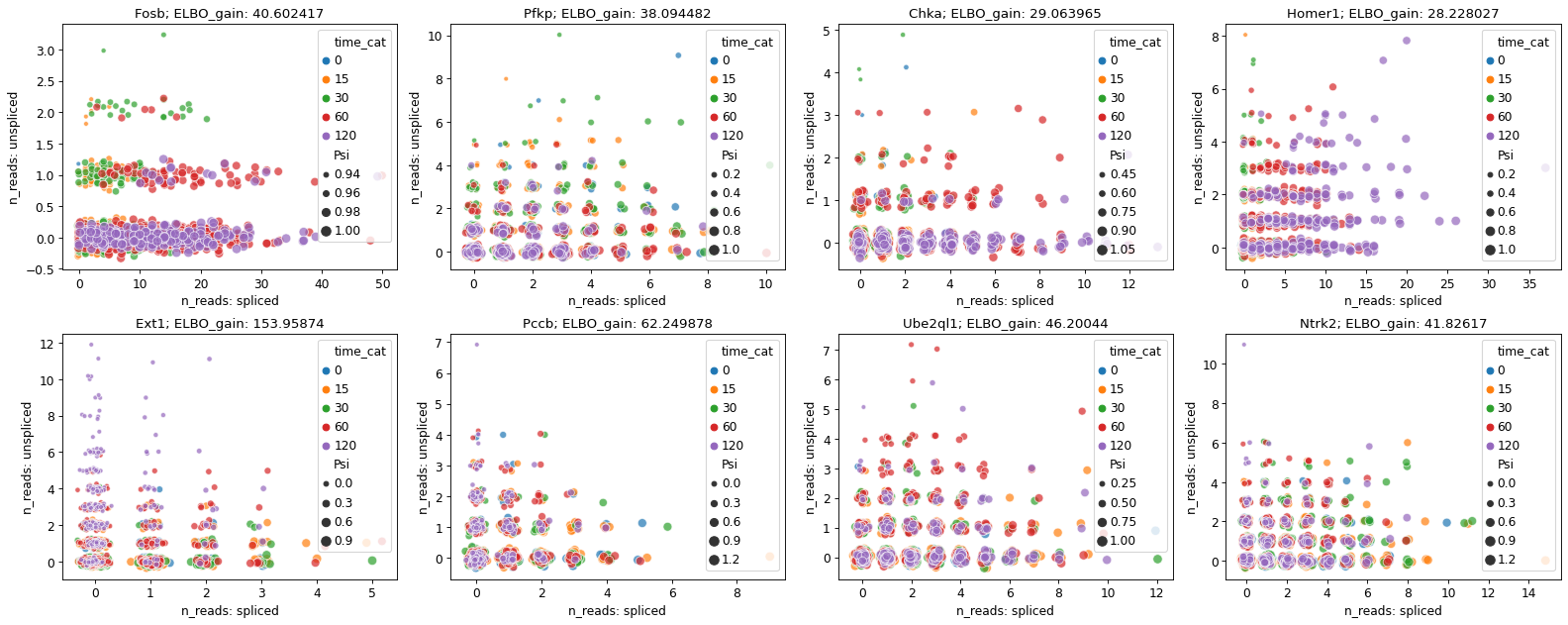
[17]:
adata_brie.obs['time_cat'] = adata_brie.obs['time'].astype('category')

gene_top_neg = ['Ext1', 'Pccb', 'Ube2ql1', 'Ntrk2']
gene_top_pos = ['Fosb', 'Pfkp', 'Chka', 'Homer1']

fig = plt.figure(figsize=(20, 8), dpi=40)
brie.pl.counts(adata_brie, genes=gene_top_pos + gene_top_neg,
               layers=['spliced', 'unspliced'],
               color='time_cat', add_val='ELBO_gain',
               nrow=2, alpha=0.7, legend='brief', noise_scale=0.1)

# plt.savefig(dat_dir + '../../figures/scNT_DMG_counts.png', dpi=150)
# plt.show()
[15]:
adata_brie[:, gene_top_pos + gene_top_neg].varm['cell_coeff']
[15]:
ArrayView([[ 0.0196298 ],
           [ 0.01087456],
           [ 0.01594826],
           [ 0.00791929],
           [-0.03045544],
           [-0.0186206 ],
           [-0.01236648],
           [-0.01042797]], dtype=float32)
[16]:
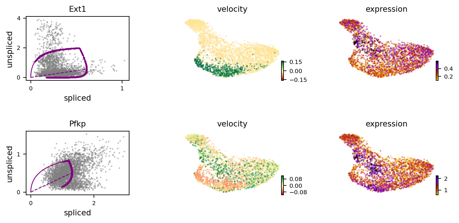
scv.pl.velocity(adata, var_names=['Ext1', 'Pfkp'], colorbar=True, ncols=1)
[ ]: