Dentate Gyrus
This processed Dentate Gyrus data set is downloaded from scVelo package, which is a very nice tool for RNA velocity quantification. Here, we will illustrate that the differential momentum genes could reveal biological informed trajectory, thanks to its supervised manner on informative gene detection.
You can run this notebook with our pre-computed data with these BRIE2 command lines, by downloading it e.g., using the following command line and unzip it into the ./data folder:
wget http://ufpr.dl.sourceforge.net/project/brie-rna/examples/dentateGyrus/brie2_dentateGyrus.zip
unzip -j brie2_dentateGyrus.zip -d ./data
Load packages
[1]:
import brie
import numpy as np
import scanpy as sc
import scvelo as scv
import matplotlib.pyplot as plt

scv.logging.print_version()
print('brie version: %s' %brie.__version__)
Running scvelo 0.2.1 (python 3.7.6) on 2020-11-06 11:53.
WARNING: There is a newer scvelo version available on PyPI:
 Your version:           0.2.1
 Latest version:         modeling
brie version: 2.0.5
[2]:
scv.settings.verbosity = 3  # show errors(0), warnings(1), info(2), hints(3)
scv.settings.presenter_view = True  # set max width size for presenter view
scv.set_figure_params('scvelo')  # for beautified visualization
[3]:
# define the path you store the example data
dat_dir = "./data"
# dat_dir = "/home/yuanhua/research/brie2/releaseDat/dentateGyrus/"
scVelo’s default results
Fitting scVelo
Scvelo’s stochastic and dynamical models may take a few minutes to run, so we pre-run it by the following codes, and the fitted data can be found in the downloaded zip file.
Stochastic model
adata = scv.datasets.dentategyrus()

scv.pp.filter_and_normalize(adata, min_shared_counts=30, n_top_genes=3000)
scv.pp.moments(adata, n_pcs=30, n_neighbors=30)

scv.tl.velocity(adata)
scv.tl.velocity_graph(adata)
adata.write(dat_dir + "/dentategyrus_scvelo_stoc_3K.h5ad")
[4]:
adata = scv.read(dat_dir + "/dentategyrus_scvelo_stoc_3K.h5ad")
[5]:
scv.utils.show_proportions(adata)
adata
Abundance of ['spliced', 'unspliced']: [0.9 0.1]
[5]:
AnnData object with n_obs × n_vars = 2930 × 2894
    obs: 'clusters', 'age(days)', 'clusters_enlarged', 'initial_size_unspliced', 'initial_size_spliced', 'initial_size', 'n_counts', 'velocity_self_transition'
    var: 'velocity_gamma', 'velocity_r2', 'velocity_genes'
    uns: 'clusters_colors', 'neighbors', 'pca', 'velocity_graph', 'velocity_graph_neg', 'velocity_params'
    obsm: 'X_pca', 'X_umap'
    varm: 'PCs'
    layers: 'Ms', 'Mu', 'ambiguous', 'spliced', 'unspliced', 'variance_velocity', 'velocity'
    obsp: 'connectivities', 'distances'
[6]:
print(np.sum(adata.var['velocity_genes']))
634
[7]:
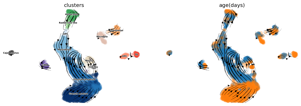
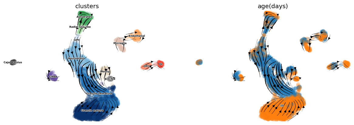
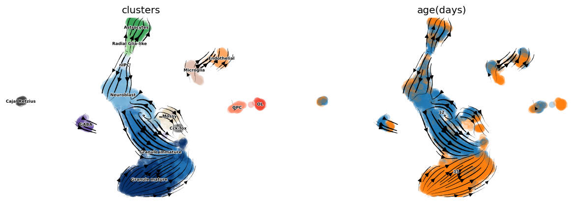
scv.tl.velocity_graph(adata, gene_subset=None)
scv.pl.velocity_embedding_stream(adata, basis='umap',
                                 color=['clusters', 'age(days)'],
                                 legend_fontsize=5, dpi=60)
computing velocity graph
    finished (0:00:04) --> added
    'velocity_graph', sparse matrix with cosine correlations (adata.uns)
computing velocity embedding
    finished (0:00:00) --> added
    'velocity_umap', embedded velocity vectors (adata.obsm)
[8]:
## Plotting with higher figure resolution

# scv.pl.velocity_embedding_stream(adata, basis='umap', color=['clusters'],
#                                  legend_fontsize=5, dpi=150, title='')

# scv.pl.velocity_embedding(adata, basis='umap', arrow_length=2, arrow_size=2, dpi=300, title='')
[ ]:
BRIE2’s differential momentum genes (DMGs)
Here, we aim to use BRIE2 to detect the differential momentum genes between cell types and illustrate its performance on projecting RNA velocity to cellular transitions. The command line and design matrix are: run_brie2.sh and dentategyrus_cluster_OL.tsv.
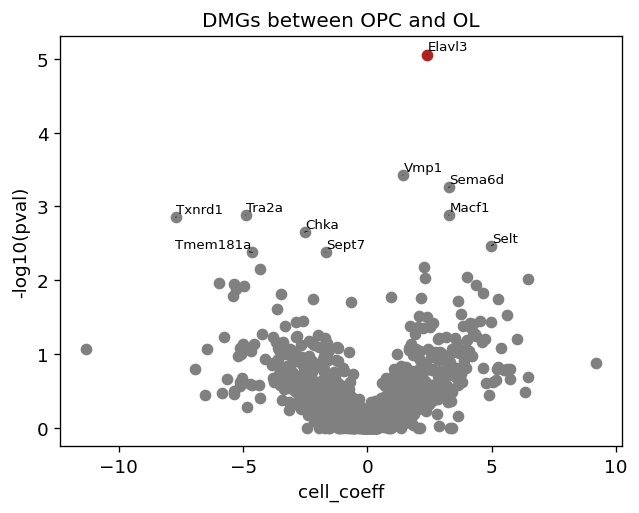
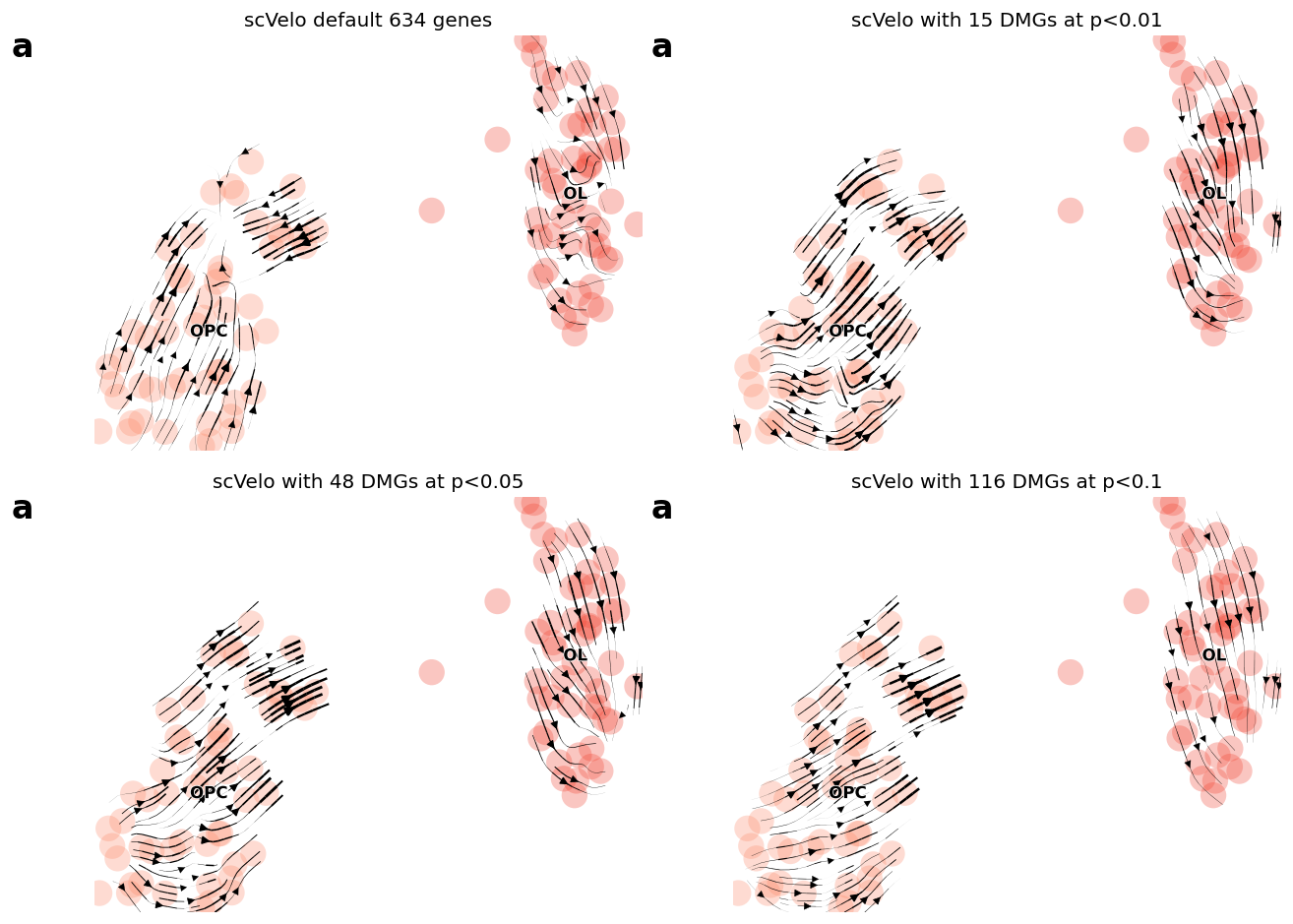
One main differentiation is between OPC and OL. So, we took out these 103 cells and run BRIE2 to detect the DMGs by testing the covariate is_OL.
[9]:
adata_brie_OL = scv.read(dat_dir + "/brie_dentategyrus_cluster_subOL.h5ad")
adata_OL = adata[adata_brie_OL.obs.index, :]
Vocalno plot for DMGs between OPC and OL. cell_ceoff means effect size on logit(Psi), Psi means proportion of spliced RNAs. Positive effect size means OL has higher proportion of spliced RNAs.
[10]:
plt.figure(figsize=(6, 4.5), dpi=60)
brie.pl.volcano(adata_brie_OL)
plt.title('DMGs between OPC and OL')
# plt.savefig(dat_dir + '../../brie2/figures/fig_s11_vocalno_DMG_OPCvsOL.pdf', dpi=150)
[10]:
Text(0.5, 1.0, 'DMGs between OPC and OL')
[11]:
top_genes_OL = adata_brie_OL.var.index[np.argsort(list(np.min(adata_brie_OL.varm['fdr'], axis=1)))[:100]]
top_genes_OL[:4]
[11]:
Index(['Elavl3', 'Sema6d', 'Vmp1', 'Tra2a'], dtype='object', name='index')
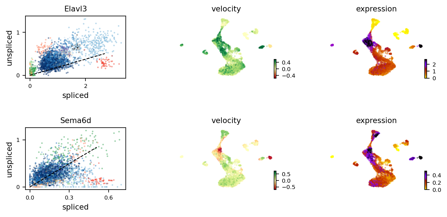
[12]:
print(adata.var['velocity_r2'][top_genes_OL[:4]])

scv.pl.velocity(adata, var_names=top_genes_OL[:2], colorbar=True, ncols=1)
index
Elavl3    0.310708
Sema6d   -0.358877
Vmp1     -0.736003
Tra2a    -1.474734
Name: velocity_r2, dtype: float64
[13]:
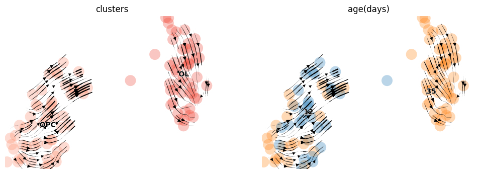
idx = adata_brie_OL.varm['ELBO_gain'][:, 0] > 2
gene_use = adata_brie_OL.var.index[idx]

print(len(gene_use), sum(brie.match(gene_use, adata_OL.var.index) != None))

scv.tl.velocity_graph(adata_OL, gene_subset=gene_use)
scv.pl.velocity_embedding_stream(adata_OL, basis='umap',
                                 color=['clusters', 'age(days)'],
                                 legend_fontsize=10, dpi=50, size=1000)
48 48
computing velocity graph
... 100%
Trying to set attribute `.uns` of view, copying.
    finished (0:00:00) --> added
    'velocity_graph', sparse matrix with cosine correlations (adata.uns)
computing velocity embedding
    finished (0:00:00) --> added
    'velocity_umap', embedded velocity vectors (adata.obsm)
[14]:
fig = plt.figure(figsize=(11, 8), dpi=60)
## cutoff 0.001
ax1 = plt.subplot(2, 2, 1)

print(np.sum(adata_OL.var['velocity_genes']))
idx1 = adata_OL.var['velocity_genes']
scv.tl.velocity_graph(adata_OL, gene_subset=None)
scv.pl.velocity_embedding_stream(adata_OL, basis='umap', color=['clusters'],
                                 ax=ax1, show=False, legend_fontsize=10,
                                 size=1000, title='scVelo default %d genes' %(sum(idx1)))
ax1.text(-0.15, 0.95, 'a', transform=ax1.transAxes, size=20, weight='bold')

## cutoff 0.05
ax1 = plt.subplot(2, 2, 2)
idx1 = adata_brie_OL.varm['pval'][:, 0] < 0.01
gene_use1 = adata_brie_OL.var.index[idx1]
print(sum(idx1), sum(brie.match(gene_use1, adata_OL.var.index) != None))

scv.tl.velocity_graph(adata_OL, gene_subset=gene_use1)
scv.pl.velocity_embedding_stream(adata_OL, basis='umap', color=['clusters'],
                                 ax=ax1, show=False, legend_fontsize=10,
                                 size=1000, title='scVelo with %d DMGs at p<0.01' %(sum(idx1)))
ax1.text(-0.15, 0.95, 'a', transform=ax1.transAxes, size=20, weight='bold')

## cutoff 0.05
ax1 = plt.subplot(2, 2, 3)

idx1 = adata_brie_OL.varm['pval'][:, 0] < 0.05
gene_use1 = adata_brie_OL.var.index[idx1]
print(sum(idx1), sum(brie.match(gene_use1, adata_OL.var.index) != None))

scv.tl.velocity_graph(adata_OL, gene_subset=gene_use1)
scv.pl.velocity_embedding_stream(adata_OL, basis='umap', color=['clusters'],
                                 ax=ax1, show=False, legend_fontsize=10,
                                 size=1000, title='scVelo with %d DMGs at p<0.05' %(sum(idx1)))
ax1.text(-0.15, 0.95, 'a', transform=ax1.transAxes, size=20, weight='bold')

## cutoff 0.05
ax1 = plt.subplot(2, 2, 4)
idx1 = adata_brie_OL.varm['pval'][:, 0] < 0.1
gene_use1 = adata_brie_OL.var.index[idx1]
print(sum(idx1), sum(brie.match(gene_use1, adata_OL.var.index) != None))

scv.tl.velocity_graph(adata_OL, gene_subset=gene_use1)
scv.pl.velocity_embedding_stream(adata_OL, basis='umap', color=['clusters'],
                                 ax=ax1, show=False, legend_fontsize=10,
                                 size=1000, title='scVelo with %d DMGs at p<0.1' %(sum(idx1)))
ax1.text(-0.15, 0.95, 'a', transform=ax1.transAxes, size=20, weight='bold')


plt.tight_layout()
# plt.savefig(dat_dir + '../../brie2/figures/fig_s12_OPLvsOL_direction.png', dpi=300)
plt.show()
634
computing velocity graph
    finished (0:00:00) --> added
    'velocity_graph', sparse matrix with cosine correlations (adata.uns)
computing velocity embedding
    finished (0:00:00) --> added
    'velocity_umap', embedded velocity vectors (adata.obsm)
15 15
computing velocity graph
    finished (0:00:00) --> added
    'velocity_graph', sparse matrix with cosine correlations (adata.uns)
computing velocity embedding
    finished (0:00:00) --> added
    'velocity_umap', embedded velocity vectors (adata.obsm)
48 48
computing velocity graph
    finished (0:00:00) --> added
    'velocity_graph', sparse matrix with cosine correlations (adata.uns)
computing velocity embedding
    finished (0:00:00) --> added
    'velocity_umap', embedded velocity vectors (adata.obsm)
116 116
computing velocity graph
    finished (0:00:00) --> added
    'velocity_graph', sparse matrix with cosine correlations (adata.uns)
computing velocity embedding
    finished (0:00:00) --> added
    'velocity_umap', embedded velocity vectors (adata.obsm)
[ ]:
We then detect the DMGs for each cell type vs the rest and use them to explore their impact on cellular transitions.
[15]:
adata_brie = scv.read(dat_dir + "/brie_dentategyrus_cluster.h5ad")
cdr = np.array((adata_brie.X > 0).mean(0))[0, :]

adata_brie
[15]:
AnnData object with n_obs × n_vars = 2930 × 2879
    obs: 'clusters', 'age(days)', 'clusters_enlarged', 'initial_size_spliced', 'initial_size_unspliced', 'initial_size'
    var: 'n_counts', 'n_counts_uniq', 'loss_gene'
    uns: 'Xc_ids', 'brie_losses', 'brie_param', 'brie_version', 'clusters_colors'
    obsm: 'X_umap', 'Xc'
    varm: 'ELBO_gain', 'cell_coeff', 'fdr', 'intercept', 'pval', 'sigma'
    layers: 'Psi', 'Psi_95CI', 'Z_std', 'ambiguous', 'spliced', 'unspliced'
[16]:
top_genes_brie = adata_brie.var.index[np.argsort(list(np.min(adata_brie.varm['fdr'], axis=1)))[:100]]
top_genes_brie[:4]
[16]:
Index(['Celf2', 'Vmp1', 'Myl6', 'Snap25'], dtype='object', name='index')
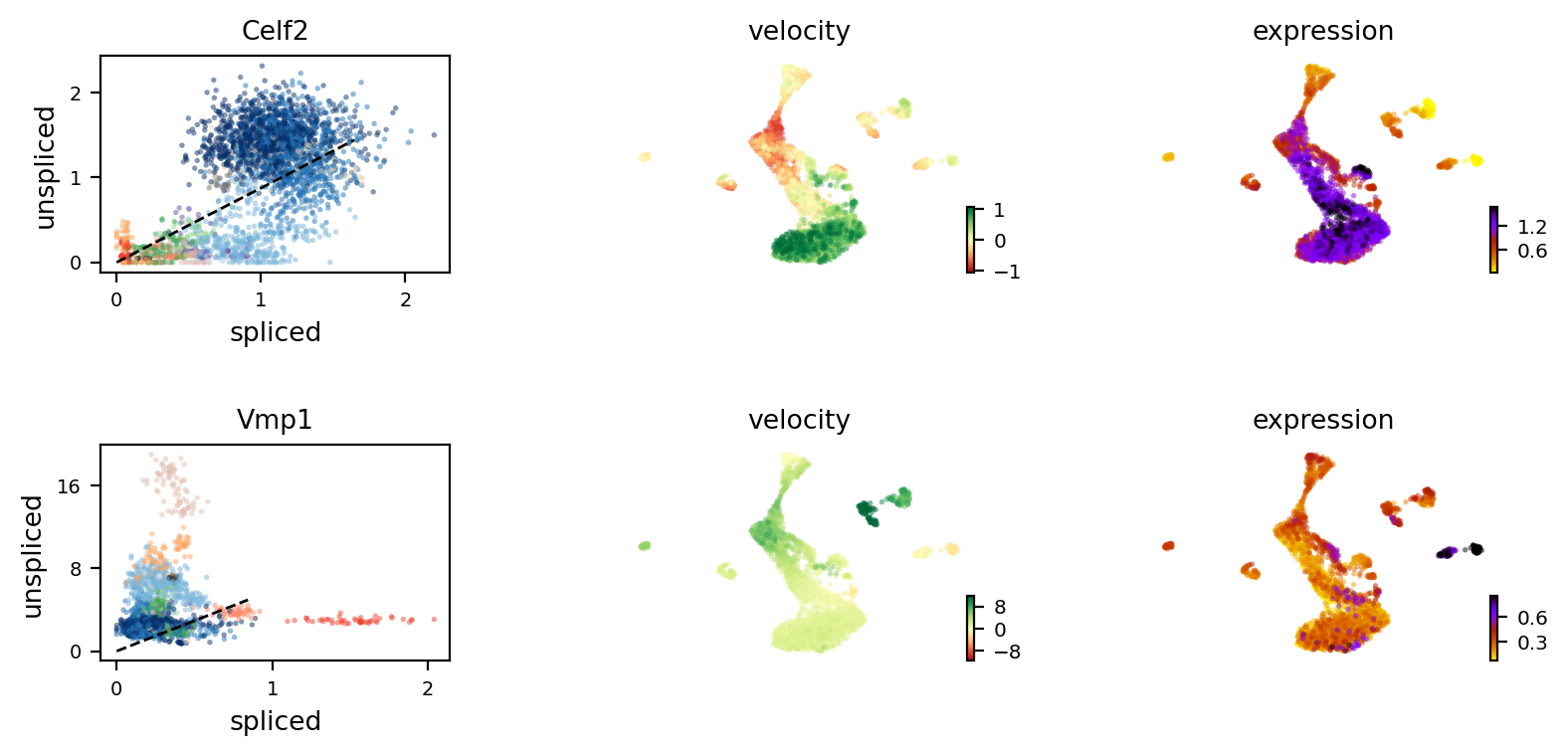
[17]:
print(adata.var['velocity_r2'][top_genes_brie[:4]])
scv.pl.velocity(adata, var_names=top_genes_brie[:2], colorbar=True, ncols=1)
index
Celf2     0.318048
Vmp1     -0.736003
Myl6      0.338808
Snap25   -0.970810
Name: velocity_r2, dtype: float64
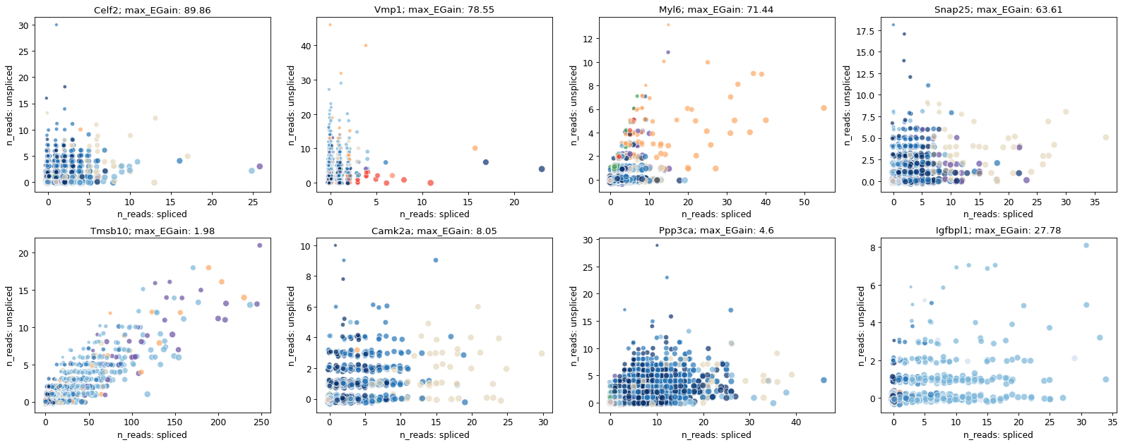
[18]:
import seaborn as sns

scVelo_genes = ['Tmsb10', 'Camk2a', 'Ppp3ca', 'Igfbpl1']
adata_brie.varm['max_EGain'] = np.round(np.max(adata_brie.varm['ELBO_gain'], axis=1, keepdims=True), 2)

fig = plt.figure(figsize=(20, 8), dpi=40)
brie.pl.counts(adata_brie, genes=np.append(top_genes_brie[:4], scVelo_genes),
               layers=['spliced', 'unspliced'],
               color='clusters', add_val='max_EGain',
               nrow=2, alpha=0.7, legend=False,
               palette=sns.color_palette(adata_brie.uns['clusters_colors']),
               hue_order=np.unique(adata_brie.obs['clusters']), noise_scale=0.1)

# plt.savefig(dat_dir + '../../brie2/figures/fig_s10_DMG_counts.png', dpi=200)
plt.show()
[19]:
idx = (np.min(adata_brie.varm['fdr'], axis=1) < 0.05) * (cdr > 0.15)
gene_use = adata_brie.var.index[idx]

print(len(gene_use), sum(brie.match(gene_use, adata.var.index) != None))

scv.tl.velocity_graph(adata, gene_subset=gene_use)
scv.pl.velocity_embedding_stream(adata, basis='umap',
                                 color=['clusters', 'age(days)'],
                                 legend_fontsize=5, dpi=60)
335 335
computing velocity graph
    finished (0:00:02) --> added
    'velocity_graph', sparse matrix with cosine correlations (adata.uns)
computing velocity embedding
    finished (0:00:00) --> added
    'velocity_umap', embedded velocity vectors (adata.obsm)
[20]:
## Plotting with higher figure resolution

# scv.pl.velocity_embedding_stream(adata, basis='umap', color=['clusters'],
#                                  legend_fontsize=5, dpi=150, title='')

# scv.pl.velocity_embedding(adata, basis='umap', arrow_length=2, arrow_size=2, dpi=300, title='')
[ ]:
scVelo’s dynamical model
Dynamical model
adata = scv.datasets.dentategyrus()

scv.pp.filter_and_normalize(adata, min_shared_counts=30, n_top_genes=3000)
scv.pp.moments(adata, n_pcs=30, n_neighbors=30)

scv.tl.recover_dynamics(adata, var_names='all')
scv.tl.velocity(adata, mode='dynamical')
scv.tl.velocity_graph(adata)
scv.tl.latent_time(adata)
adata.write(dat_dir + "/dentategyrus_scvelo_dyna_3K.h5ad")
[21]:
adata_dyna = scv.read(dat_dir + "/dentategyrus_scvelo_dyna_3K.h5ad")
[22]:
print(np.sum(adata_dyna.var['velocity_genes']))
1066
[23]:
# scv.tl.velocity_graph(adata_dyna, gene_subset=None)
scv.pl.velocity_embedding_stream(adata_dyna, basis='umap',
                                 color=['clusters', 'age(days)'],
                                 legend_fontsize=5, dpi=60)
computing velocity embedding
    finished (0:00:00) --> added
    'velocity_umap', embedded velocity vectors (adata.obsm)
[ ]: